ST558_Project-2
Modeling the rental count of bikes _ Main code
Mu-Tien, Lee
- Require package
- Read in data
- Summarize the training data
- Training Model
- Predicting using the best tree-base model
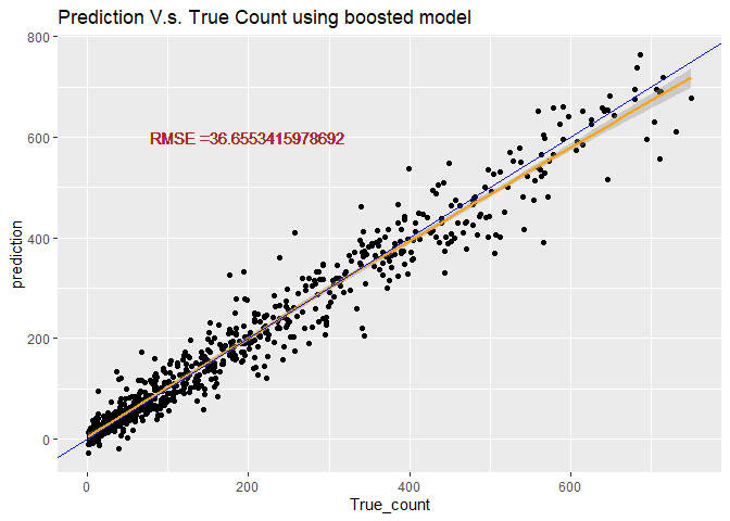
- Predicting using the best boosted-tree model
Require package
#install.packages("")
library(knitr)
library(rmarkdown)
library(MuMIn)
library(tidyverse)
library(caret)
library(corrplot)
library(readxl)
library(caret)
library(ggiraphExtra)
library(knitr)
library(ggplot2)
library(ggpubr)
library(rpart.plot)
library(rpart)
library(DT)
Read in data
#read in hour data
HourData <- read.csv("hour.csv")
HourData<- HourData %>% select(-casual, -registered)
HourData$yr <- as.factor(HourData$yr)
HourData$holiday <- as.factor(HourData$holiday)
HourData$workingday <- as.factor(HourData$workingday)

#filter data by weekday
HourData <-HourData %>% filter(weekday==params$w)
#showing data
HourData <-HourData %>% select(-weekday, -workingday,-instant)
tbl_df(HourData)
## # A tibble: 2,512 x 12
##    dteday season yr     mnth    hr holiday weathersit  temp atemp   hum
##    <chr>   <int> <fct> <int> <int> <fct>        <int> <dbl> <dbl> <dbl>
##  1 2011-~      1 0         1     0 0                1  0.24 0.288  0.81
##  2 2011-~      1 0         1     1 0                1  0.22 0.273  0.8
##  3 2011-~      1 0         1     2 0                1  0.22 0.273  0.8
##  4 2011-~      1 0         1     3 0                1  0.24 0.288  0.75
##  5 2011-~      1 0         1     4 0                1  0.24 0.288  0.75
##  6 2011-~      1 0         1     5 0                2  0.24 0.258  0.75
##  7 2011-~      1 0         1     6 0                1  0.22 0.273  0.8
##  8 2011-~      1 0         1     7 0                1  0.2  0.258  0.86
##  9 2011-~      1 0         1     8 0                1  0.24 0.288  0.75
## 10 2011-~      1 0         1     9 0                1  0.32 0.348  0.76
## # ... with 2,502 more rows, and 2 more variables: windspeed <dbl>, cnt <int>
#Separate dataset into train (70%) and test (30%) data set
set.seed(1997)
train <- sample(1:nrow(HourData), size = nrow(HourData)*0.7)
test <- dplyr::setdiff(1:nrow(HourData), train)
HourDataTrain <- HourData[train, ]
HourDataTest <- HourData[test, ]
Summarize the training data
Here I will show you some summary of my training dataset.
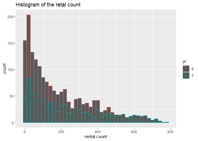
1. I conduct a histogram of the rental count, since this is my response
variable.
2. I built up a summary table of all the weather measurement.
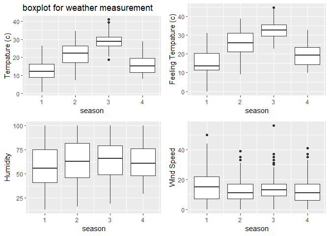
3. I also showing the weather summary via a boxplot.
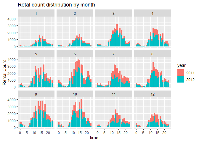
4. I plot the rental count distributed by time.
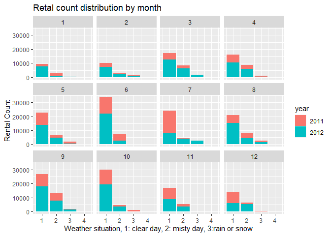
5. I plot the rental count distributed by weather situation.
# plot the histogram of rental count
hist <- ggplot(data=HourDataTrain, aes(x=cnt))+geom_histogram(binwidth = 20, aes(color=yr))
hist <-hist+labs(title="Histogram of the retal count", x="rental count")
hist <-hist+scale_fill_discrete(labels=c(2011,2012))
hist
#prin out summary table for tempature humidity and windspeed
sum <- HourDataTrain%>% select(c(temp, atemp, hum, windspeed))
kable(apply(sum, 2,summary), caption="Numeric Summary for weather measurement")
| temp | atemp | hum | windspeed | |
|---|---|---|---|---|
| Min. | 0.0200000 | 0.0000000 | 0.1300000 | 0.0000000 |
| 1st Qu. | 0.3200000 | 0.3030000 | 0.4500000 | 0.1045000 |
| Median | 0.4600000 | 0.4545000 | 0.6200000 | 0.1940000 |
| Mean | 0.4828441 | 0.4628265 | 0.6169113 | 0.1979813 |
| 3rd Qu. | 0.6400000 | 0.6212000 | 0.7800000 | 0.2836000 |
| Max. | 1.0000000 | 0.8939000 | 1.0000000 | 0.8358000 |
Numeric Summary for weather measurement
#plot the boxplot of tempature humidity and windspeed (not genralized amount)
#plot base
boxplot <- ggplot(data = HourDataTrain, aes(x=season))
#adding 4 variables
tem <-boxplot+geom_boxplot(aes(y=temp*41, group=season))+labs(y="Tempature (c)", title = "boxplot for weather measurement")
fetem <-boxplot+geom_boxplot(aes(y=atemp*50, group=season))+labs(y="Feeling Tempature (c)")
hum <-boxplot+geom_boxplot(aes(y=hum*100, group=season))+labs(y="Humidity")
wind <-boxplot+geom_boxplot(aes(y=windspeed*67, group=season))+labs(y="Wind Speed")
#combine 4 plots into 1
ggarrange(tem, fetem, hum , wind, ncol = 2, nrow = 2)
# plot the count distribution among time and weather
# by time
barplot1<-ggplot(data = HourDataTrain, aes(x=hr))+geom_col(aes(y=cnt, fill=yr))+facet_wrap(~mnth)
barplot1 <- barplot1+labs(x="time", y="Rental Count", title="Retal count distribution by month" )
barplot1+scale_fill_discrete(name="year", labels=c(2011,2012))
# by weather
barplot2 <-ggplot(data = HourDataTrain, aes(x=weathersit))+geom_col(aes(y=cnt, fill=yr))+facet_wrap(~mnth)
barplot2 <- barplot2+labs(x="Weather situation, 1: clear day, 2: misty day, 3:rain or snow", y="Rental Count", title="Retal count distribution by month" )
barplot2+scale_fill_discrete(name="year", labels=c(2011,2012))
Training Model
Here I use two different method to train my model. First method is using
a tree-based models with leave one out cross validation. For the second
method, I use the boosted tree model with cross validation. Both two
training are done using the train function from caret package. The
data was cantered and scaled before training.
Tree-based model
Since our respons variable is continuous. I use the regression tree
model to training my data. The method= "rpart" was used in train
function
Moreover, because I want to use the leave-one-out cross validation for
this training, therefore,the method= "LOOCV" was used in
trainControl.
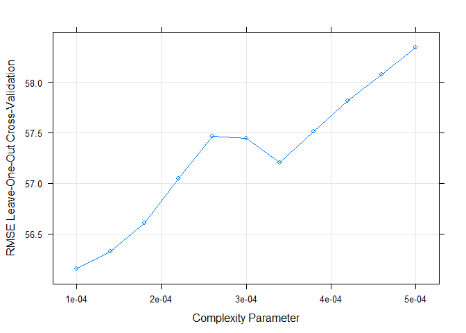
We can adjust the grid parameter by ourselves. Since the default result
shows that cp should be very small to have a lowest RMSE. I set a
range [0.0001,0.0005] to fit for every weekday.
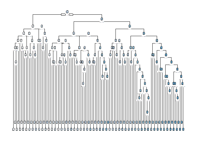
Something to notice, because the cp is too small, when I draw my
regression tree, it seems like a mess.
# set up training control, using leave one out cross validation.
set.seed(615)
trctrl <- trainControl(method = "LOOCV", number = 1)

# getModelInfo("rpart")
# training using regression tree models with cp in [0.0001,0.0005]
# since the cp seems have to be really small when I used the default cp to train

model1 <- cnt~season+yr+mnth+hr+holiday+weathersit+temp+atemp+hum+windspeed

RegTree_fit1 <- train(model1, data = HourDataTrain, method = "rpart",
                 trControl=trctrl,
                 preProcess = c("center", "scale"),
                 tuneGrid=expand.grid(cp=seq(0.0001,0.0005,0.00004))
)

# show the training result
RegTree_fit1
## CART
##
## 1758 samples
##   10 predictor
##
## Pre-processing: centered (10), scaled (10)
## Resampling: Leave-One-Out Cross-Validation
## Summary of sample sizes: 1757, 1757, 1757, 1757, 1757, 1757, ...
## Resampling results across tuning parameters:
##
##   cp       RMSE      Rsquared   MAE
##   0.00010  56.15857  0.9028623  37.24338
##   0.00014  56.32850  0.9022547  37.77139
##   0.00018  56.60765  0.9013206  38.11030
##   0.00022  57.04474  0.8997897  38.72014
##   0.00026  57.46700  0.8982885  39.18662
##   0.00030  57.44314  0.8982776  39.14039
##   0.00034  57.20356  0.8990944  38.81209
##   0.00038  57.51070  0.8979730  39.06176
##   0.00042  57.81257  0.8969561  39.38842
##   0.00046  58.07947  0.8960387  39.64212
##   0.00050  58.34052  0.8951472  39.75799
##
## RMSE was used to select the optimal model using the smallest value.
## The final value used for the model was cp = 1e-04.
# plot the RMSE of selected cp
plot(RegTree_fit1)
# plot my final tree model
rpart.plot(RegTree_fit1$finalModel)
Boosted tree model
Here I want to training my data using boosted tree model. The method=
"gbm" was used in train function
Because I want to use thecross validation for this training,
therefore,the method= "cv" was used in trainControl.
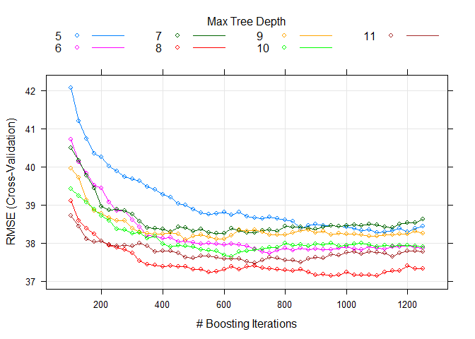
We can adjust the grid parameter by ourselves. I set a range of number
of tree [100,1250] and interaction 5~11 to fit for every weekday.
# set up training control, using cross validation with 10 folder
set.seed(615)
trctrl <- trainControl(method = "cv", number = 10)

# training using boosted tree models with boosting interation in [700,1250] and try max tree depth 5~9
model2 <- cnt~season+yr+mnth+hr+holiday+weathersit+temp+atemp+hum+windspeed
RegTree_fit2 <- train(model2, data = HourDataTrain, method = "gbm",
                trControl=trctrl,
                preProcess = c("center", "scale"),
                tuneGrid=expand.grid(n.trees=seq(100,1250,25),
                                     interaction.depth=5:11,
                                     shrinkage=0.1, n.minobsinnode=10)
                 )
# show the training result of boosted tree
RegTree_fit2$bestTune
##     n.trees interaction.depth shrinkage n.minobsinnode
## 176     950                 8       0.1             10
# plot the RMSE of different parameters
plot(RegTree_fit2)
Predicting using the best tree-base model
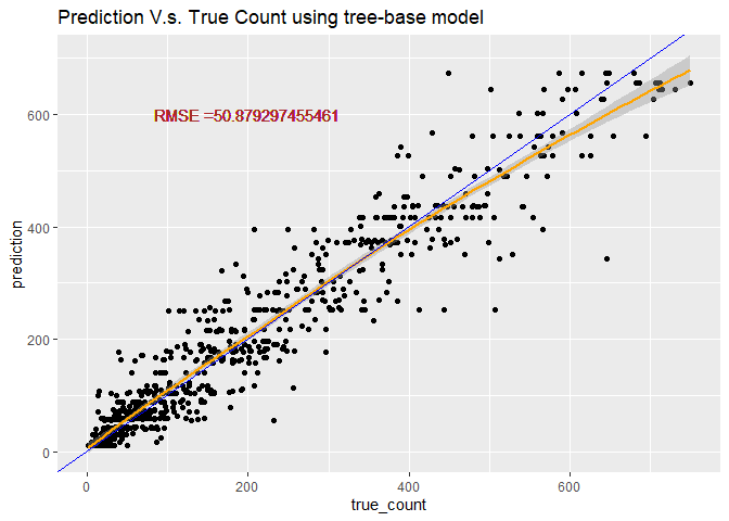
Using the best boosted tree model to testing the data.
# predict use predict function
tree_pred <- predict(RegTree_fit1, newdata = HourDataTest)

#Calculate the Root MSE
RMSE_tree<- sqrt(mean((tree_pred-HourDataTest$cnt)^2))
label <- paste0("RMSE =", RMSE_tree)

# plot the prediction
count <- data.frame(true_count=HourDataTest$cnt,prediction=tree_pred )
predPlot <- ggplot(data=count, aes(x=true_count,y=prediction))
predPlot <- predPlot+labs(title="Prediction V.s. True Count using tree-base model")+geom_point()
predPlot <- predPlot+geom_smooth(color="orange")+geom_abline(aes(intercept=0,slope=1), color="blue")
predPlot <- predPlot+geom_text(x=200, y=600,label=label, color="brown")
predPlot
Predicting using the best boosted-tree model
# predict use predict function
boosted_pred <- predict(RegTree_fit2, newdata = HourDataTest)

#Calculate the Root MSE
RMSE_boosted <- sqrt(mean((boosted_pred-HourDataTest$cnt)^2))
lab <- paste0("RMSE =", RMSE_boosted)
# plot the prediction
count2 <- data.frame(True_count=HourDataTest$cnt,prediction=boosted_pred )
pred_plot <- ggplot(data=count2, aes(x=True_count,y=prediction))
pred_plot <- pred_plot+labs(title="Prediction V.s. True Count using boosted model")+geom_point()
pred_plot <- pred_plot+geom_smooth(color="orange")+geom_abline(aes(intercept=0,slope=1), color="blue")
pred_plot <- pred_plot+geom_text(x=200, y=600,label=lab, color=" brown")
pred_plot
# create a linear model using repeated cross-validation
linear_mod <- train(cnt~season+yr+mnth+hr+holiday+weathersit+temp+atemp+hum+windspeed,
                    data=HourDataTrain,
                    method='lm',
                    preProcess=c("center", "scale"),
                    metric='RMSE',
                    tuneLength=10,
                    trControl=trainControl(method='repeatedcv', number=10, repeats=3)
                    )

# display the results of the linear model
summary(linear_mod)
##
## Call:
## lm(formula = .outcome ~ ., data = dat)
##
## Residuals:
##     Min      1Q  Median      3Q     Max
## -298.30  -90.98   -6.49   75.15  442.68
##
## Coefficients: (1 not defined because of singularities)
##             Estimate Std. Error t value Pr(>|t|)
## (Intercept) 191.0580     2.9651  64.436  < 2e-16 ***
## season       24.8097     5.0613   4.902 1.04e-06 ***
## yr1          39.9551     2.9887  13.369  < 2e-16 ***
## mnth         -5.3766     4.9135  -1.094  0.27399
## hr           44.7120     3.1308  14.281  < 2e-16 ***
## holiday1          NA         NA      NA       NA
## weathersit   10.7246     3.4782   3.083  0.00208 **
## temp        -69.7246    25.7870  -2.704  0.00692 **
## atemp       143.4024    25.8255   5.553 3.24e-08 ***
## hum         -61.7855     3.7425 -16.509  < 2e-16 ***
## windspeed     0.4153     3.3536   0.124  0.90146
## ---
## Signif. codes:  0 '***' 0.001 '**' 0.01 '*' 0.05 '.' 0.1 ' ' 1
##
## Residual standard error: 124.3 on 1748 degrees of freedom
## Multiple R-squared:  0.5244, Adjusted R-squared:  0.522
## F-statistic: 214.2 on 9 and 1748 DF,  p-value: < 2.2e-16
# compare our linear model to our test data
linear_pred <- predict(linear_mod, newdata=HourDataTest)
postResample(linear_pred, HourDataTest$cnt)
##        RMSE    Rsquared         MAE
## 119.6701206   0.5576787  93.5003677