ST558_Project-2
Modeling the rental count of bikes _ Main code
Mu-Tien, Lee
- Require package
- Read in data
- Summarize the training data
- Training Model
- Predicting using the best tree-base model
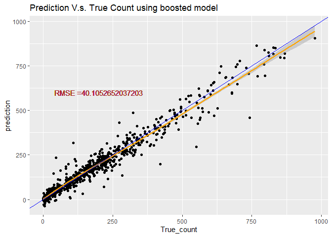
- Predicting using the best boosted-tree model
Require package
#install.packages("")
library(knitr)
library(rmarkdown)
library(MuMIn)
library(tidyverse)
library(caret)
library(corrplot)
library(readxl)
library(caret)
library(ggiraphExtra)
library(knitr)
library(ggplot2)
library(ggpubr)
library(rpart.plot)
library(rpart)
library(DT)
Read in data
#read in hour data
HourData <- read.csv("hour.csv")
HourData<- HourData %>% select(-casual, -registered)
HourData$yr <- as.factor(HourData$yr)
HourData$holiday <- as.factor(HourData$holiday)
HourData$workingday <- as.factor(HourData$workingday)

#filter data by weekday
HourData <-HourData %>% filter(weekday==params$w)
#showing data
HourData <-HourData %>% select(-weekday, -workingday,-instant)
tbl_df(HourData)
## # A tibble: 2,471 x 12
##    dteday season yr     mnth    hr holiday weathersit  temp atemp   hum
##    <chr>   <int> <fct> <int> <int> <fct>        <int> <dbl> <dbl> <dbl>
##  1 2011-~      1 0         1     0 0                1  0.18 0.242  0.55
##  2 2011-~      1 0         1     1 0                1  0.16 0.227  0.64
##  3 2011-~      1 0         1     2 0                1  0.16 0.227  0.64
##  4 2011-~      1 0         1     4 0                2  0.16 0.197  0.64
##  5 2011-~      1 0         1     5 0                2  0.14 0.182  0.69
##  6 2011-~      1 0         1     6 0                2  0.14 0.167  0.63
##  7 2011-~      1 0         1     7 0                2  0.16 0.227  0.59
##  8 2011-~      1 0         1     8 0                1  0.16 0.227  0.59
##  9 2011-~      1 0         1     9 0                2  0.18 0.242  0.51
## 10 2011-~      1 0         1    10 0                1  0.2  0.258  0.47
## # ... with 2,461 more rows, and 2 more variables: windspeed <dbl>, cnt <int>
#Separate dataset into train (70%) and test (30%) data set
set.seed(1997)
train <- sample(1:nrow(HourData), size = nrow(HourData)*0.7)
test <- dplyr::setdiff(1:nrow(HourData), train)
HourDataTrain <- HourData[train, ]
HourDataTest <- HourData[test, ]
Summarize the training data
Here I will show you some summary of my training dataset.
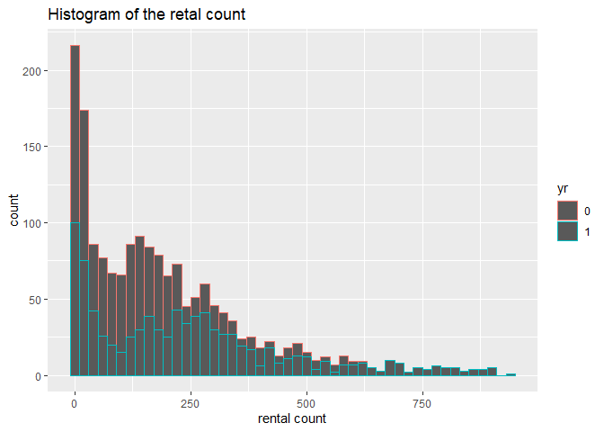
1. I conduct a histogram of the rental count, since this is my response
variable.
2. I built up a summary table of all the weather measurement.
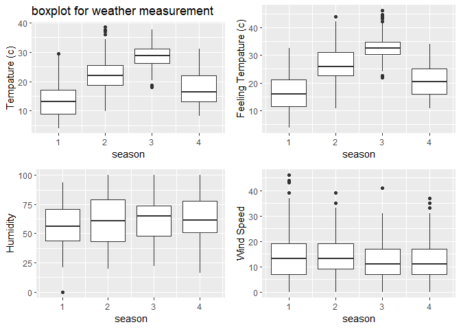
3. I also showing the weather summary via a boxplot.
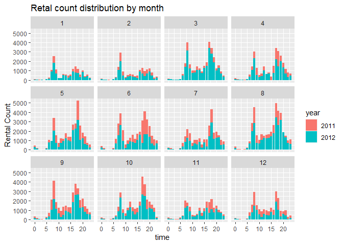
4. I plot the rental count distributed by time.
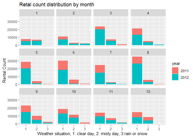
5. I plot the rental count distributed by weather situation.
# plot the histogram of rental count
hist <- ggplot(data=HourDataTrain, aes(x=cnt))+geom_histogram(binwidth = 20, aes(color=yr))
hist <-hist+labs(title="Histogram of the retal count", x="rental count")
hist <-hist+scale_fill_discrete(labels=c(2011,2012))
hist
#prin out summary table for tempature humidity and windspeed
sum <- HourDataTrain%>% select(c(temp, atemp, hum, windspeed))
kable(apply(sum, 2,summary), caption="Numeric Summary for weather measurement")
| temp | atemp | hum | windspeed | |
|---|---|---|---|---|
| Min. | 0.1000000 | 0.0758000 | 0.0000000 | 0.0000000 |
| 1st Qu. | 0.3400000 | 0.3333000 | 0.4700000 | 0.1045000 |
| Median | 0.5000000 | 0.4848000 | 0.6100000 | 0.1940000 |
| Mean | 0.5064199 | 0.4842271 | 0.6132678 | 0.1907718 |
| 3rd Qu. | 0.6600000 | 0.6212000 | 0.7700000 | 0.2537000 |
| Max. | 0.9400000 | 0.9242000 | 1.0000000 | 0.6866000 |
Numeric Summary for weather measurement
#plot the boxplot of tempature humidity and windspeed (not genralized amount)
#plot base
boxplot <- ggplot(data = HourDataTrain, aes(x=season))
#adding 4 variables
tem <-boxplot+geom_boxplot(aes(y=temp*41, group=season))+labs(y="Tempature (c)", title = "boxplot for weather measurement")
fetem <-boxplot+geom_boxplot(aes(y=atemp*50, group=season))+labs(y="Feeling Tempature (c)")
hum <-boxplot+geom_boxplot(aes(y=hum*100, group=season))+labs(y="Humidity")
wind <-boxplot+geom_boxplot(aes(y=windspeed*67, group=season))+labs(y="Wind Speed")
#combine 4 plots into 1
ggarrange(tem, fetem, hum , wind, ncol = 2, nrow = 2)
# plot the count distribution among time and weather
# by time
barplot1<-ggplot(data = HourDataTrain, aes(x=hr))+geom_col(aes(y=cnt, fill=yr))+facet_wrap(~mnth)
barplot1 <- barplot1+labs(x="time", y="Rental Count", title="Retal count distribution by month" )
barplot1+scale_fill_discrete(name="year", labels=c(2011,2012))
# by weather
barplot2 <-ggplot(data = HourDataTrain, aes(x=weathersit))+geom_col(aes(y=cnt, fill=yr))+facet_wrap(~mnth)
barplot2 <- barplot2+labs(x="Weather situation, 1: clear day, 2: misty day, 3:rain or snow", y="Rental Count", title="Retal count distribution by month" )
barplot2+scale_fill_discrete(name="year", labels=c(2011,2012))
Training Model
Here I use two different method to train my model. First method is using
a tree-based models with leave one out cross validation. For the second
method, I use the boosted tree model with cross validation. Both two
training are done using the train function from caret package. The
data was cantered and scaled before training.
Tree-based model
Since our respons variable is continuous. I use the regression tree
model to training my data. The method= "rpart" was used in train
function
Moreover, because I want to use the leave-one-out cross validation for
this training, therefore,the method= "LOOCV" was used in
trainControl.
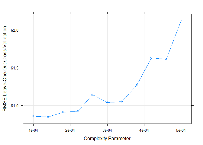
We can adjust the grid parameter by ourselves. Since the default result
shows that cp should be very small to have a lowest RMSE. I set a
range [0.0001,0.0005] to fit for every weekday.
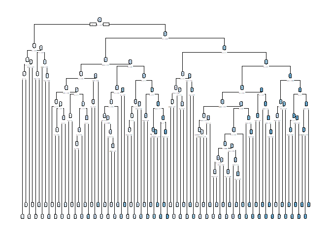
Something to notice, because the cp is too small, when I draw my
regression tree, it seems like a mess.
# set up training control, using leave one out cross validation.
set.seed(615)
trctrl <- trainControl(method = "LOOCV", number = 1)

# getModelInfo("rpart")
# training using regression tree models with cp in [0.0001,0.0005]
# since the cp seems have to be really small when I used the default cp to train

model1 <- cnt~season+yr+mnth+hr+holiday+weathersit+temp+atemp+hum+windspeed

RegTree_fit1 <- train(model1, data = HourDataTrain, method = "rpart",
                 trControl=trctrl,
                 preProcess = c("center", "scale"),
                 tuneGrid=expand.grid(cp=seq(0.0001,0.0005,0.00004))
)

# show the training result
RegTree_fit1
## CART
##
## 1729 samples
##   10 predictor
##
## Pre-processing: centered (10), scaled (10)
## Resampling: Leave-One-Out Cross-Validation
## Summary of sample sizes: 1728, 1728, 1728, 1728, 1728, 1728, ...
## Resampling results across tuning parameters:
##
##   cp       RMSE      Rsquared   MAE
##   0.00010  60.86147  0.8970593  36.61289
##   0.00014  60.84946  0.8970917  36.89877
##   0.00018  60.91024  0.8968519  37.09426
##   0.00022  60.92366  0.8967952  37.38067
##   0.00026  61.14398  0.8960384  37.95852
##   0.00030  61.03935  0.8963359  38.20563
##   0.00034  61.04983  0.8962482  38.23389
##   0.00038  61.26566  0.8955081  38.32099
##   0.00042  61.63042  0.8943369  38.68553
##   0.00046  61.60945  0.8944215  38.65511
##   0.00050  62.12086  0.8926813  39.15997
##
## RMSE was used to select the optimal model using the smallest value.
## The final value used for the model was cp = 0.00014.
# plot the RMSE of selected cp
plot(RegTree_fit1)
# plot my final tree model
rpart.plot(RegTree_fit1$finalModel)
Boosted tree model
Here I want to training my data using boosted tree model. The method=
"gbm" was used in train function
Because I want to use thecross validation for this training,
therefore,the method= "cv" was used in trainControl.
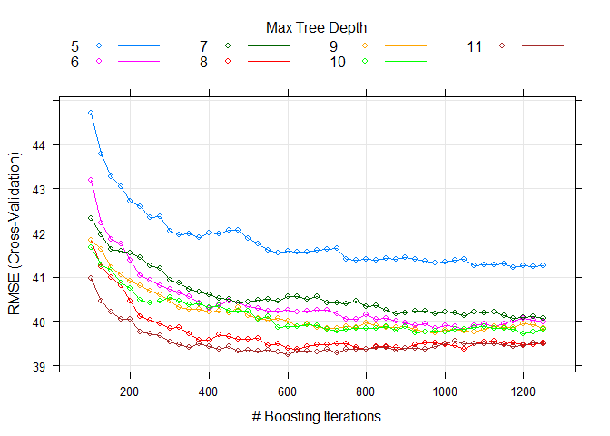
We can adjust the grid parameter by ourselves. I set a range of number
of tree [100,1250] and interaction 5~11 to fit for every weekday.
# set up training control, using cross validation with 10 folder
set.seed(615)
trctrl <- trainControl(method = "cv", number = 10)

# training using boosted tree models with boosting interation in [700,1250] and try max tree depth 5~9
model2 <- cnt~season+yr+mnth+hr+holiday+weathersit+temp+atemp+hum+windspeed
RegTree_fit2 <- train(model2, data = HourDataTrain, method = "gbm",
                trControl=trctrl,
                preProcess = c("center", "scale"),
                tuneGrid=expand.grid(n.trees=seq(100,1250,25),
                                     interaction.depth=5:11,
                                     shrinkage=0.1, n.minobsinnode=10)
                 )
# show the training result of boosted tree
RegTree_fit2$bestTune
##     n.trees interaction.depth shrinkage n.minobsinnode
## 303     600                11       0.1             10
# plot the RMSE of different parameters
plot(RegTree_fit2)
Predicting using the best tree-base model
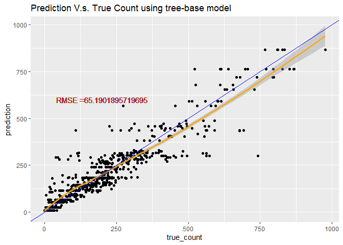
Using the best boosted tree model to testing the data.
# predict use predict function
tree_pred <- predict(RegTree_fit1, newdata = HourDataTest)

#Calculate the Root MSE
RMSE_tree<- sqrt(mean((tree_pred-HourDataTest$cnt)^2))
label <- paste0("RMSE =", RMSE_tree)

# plot the prediction
count <- data.frame(true_count=HourDataTest$cnt,prediction=tree_pred )
predPlot <- ggplot(data=count, aes(x=true_count,y=prediction))
predPlot <- predPlot+labs(title="Prediction V.s. True Count using tree-base model")+geom_point()
predPlot <- predPlot+geom_smooth(color="orange")+geom_abline(aes(intercept=0,slope=1), color="blue")
predPlot <- predPlot+geom_text(x=200, y=600,label=label, color="brown")
predPlot
Predicting using the best boosted-tree model
# predict use predict function
boosted_pred <- predict(RegTree_fit2, newdata = HourDataTest)

#Calculate the Root MSE
RMSE_boosted <- sqrt(mean((boosted_pred-HourDataTest$cnt)^2))
lab <- paste0("RMSE =", RMSE_boosted)
# plot the prediction
count2 <- data.frame(True_count=HourDataTest$cnt,prediction=boosted_pred )
pred_plot <- ggplot(data=count2, aes(x=True_count,y=prediction))
pred_plot <- pred_plot+labs(title="Prediction V.s. True Count using boosted model")+geom_point()
pred_plot <- pred_plot+geom_smooth(color="orange")+geom_abline(aes(intercept=0,slope=1), color="blue")
pred_plot <- pred_plot+geom_text(x=200, y=600,label=lab, color=" brown")
pred_plot
# create a linear model using repeated cross-validation
linear_mod <- train(cnt~season+yr+mnth+hr+holiday+weathersit+temp+atemp+hum+windspeed,
                    data=HourDataTrain,
                    method='lm',
                    preProcess=c("center", "scale"),
                    metric='RMSE',
                    tuneLength=10,
                    trControl=trainControl(method='repeatedcv', number=10, repeats=3)
                    )

# display the results of the linear model
summary(linear_mod)
##
## Call:
## lm(formula = .outcome ~ ., data = dat)
##
## Residuals:
##     Min      1Q  Median      3Q     Max
## -311.81  -95.65  -34.32   55.87  614.02
##
## Coefficients:
##             Estimate Std. Error t value Pr(>|t|)
## (Intercept)  196.011      3.668  53.440  < 2e-16 ***
## season        13.219      6.794   1.946 0.051841 .
## yr1           48.235      3.739  12.900  < 2e-16 ***
## mnth           3.302      6.562   0.503 0.614879
## hr            65.329      3.901  16.746  < 2e-16 ***
## holiday1     -16.303      3.810  -4.279 1.98e-05 ***
## weathersit   -12.985      4.001  -3.246 0.001195 **
## temp          42.614     28.458   1.497 0.134466
## atemp          3.629     28.435   0.128 0.898446
## hum          -16.561      4.330  -3.825 0.000135 ***
## windspeed     11.013      4.002   2.752 0.005984 **
## ---
## Signif. codes:  0 '***' 0.001 '**' 0.01 '*' 0.05 '.' 0.1 ' ' 1
##
## Residual standard error: 152.5 on 1718 degrees of freedom
## Multiple R-squared:  0.3551, Adjusted R-squared:  0.3514
## F-statistic: 94.61 on 10 and 1718 DF,  p-value: < 2.2e-16
# compare our linear model to our test data
linear_pred <- predict(linear_mod, newdata=HourDataTest)
postResample(linear_pred, HourDataTest$cnt)
##        RMSE    Rsquared         MAE
## 147.1752454   0.3658021 108.0946553